Beyond L-Systems
In the first part of this post, we went over Lindenmayer systems, and saw how from small sets of very simple rules, complexity emerged in the form of intricate patterns. In this part, we will look at two other types of fractals. The first one, is called the Barnsley fern, and unlike the L-systems in the previous post, it is based not on string substitution, but on the repeated iteration of affine transformations to a starting point. The second fractal we'll cover in this post is the Mandelbrot set, which may well be the "most famous" fractal out there, and for good reason, as it it really fascinating.
Between Many Ferns
The Barnsley fern is built by applying, in an iterative fashion, a series of affine transformations to a point. The transformations are chosen randomly between four possible ones, and the probability of choosing each one at each iteration is given by a fixed distribution, as follows.
| Transformation | Probability |
| $f1$ | 0.01 |
| $f2$ | 0.85 |
| $f3$ | 0.07 |
| $f4$ | 0.07 |
Each transformation has the form $Av^\intercal + w$, where $A$ is a $2\times2$ matrix, $v=(x,y)$ is the point being transformed, and $w$ is a constant vector. If $A$ is of the form $$ \begin{pmatrix} a&b \\ c&d \end{pmatrix}$$ and $w$ is of the form $$ \begin{pmatrix} e \\ f\end{pmatrix}$$ then we have $$f(x,y) = \begin{pmatrix} ax + by + e \\ cx + dy + f \end{pmatrix} $$
The coefficients for the $f1\cdots f4$ transformations are as follows:
| Transforms | Coeff. | |||||
| a | b | c | d | e | f | |
| $f1$ | 0 | 0 | 0 | 0.16 | 0 | 0 |
| $f2$ | 0.85 | 0.04 | -0.04 | 0.85 | 0 | 1.6 |
| $f3$ | 0.2 | -0.26 | 0.23 | 0.22 | 0 | 1.6 |
| $f4$ | -0.15 | 0.28 | 0.26 | 0.24 | 0 | 0.44 |
We can start putting this to code, by defining the transformations and their application:
(ns fractals.barnsley
  (:require [fractals.util :as util]    ;; We'll use a helper to scale the plot to the canvas
            [hiccup.core :as hiccup]))  ;; And hiccup to generate the HTML/SVG

(def transforms {:f1 [0 0 0 0.16 0 0]
                 :f2 [0.85 0.04 -0.04 0.85 0 1.6]
                 :f3 [0.2 -0.26 0.23 0.22 0 1.6]
                 :f4 [-0.15 0.28 0.26 0.24 0 0.44]})


(defn- apply-transform [point coeffs]
  (if (empty? coeffs)
    [0 0]
    (let [[x y] point
          [a b c d e f] coeffs
          xx  (+ (* a x) (* b y) e)
          yy  (+ (* c x) (* d y) f)]
      [xx yy])))
With that done, we can proceed to implement the actual Barnsley fern fractal. First, we pick the transformations with the given probability distribution
(defn- transform-probs [i]
  (cond
    (<= i 0.01) :f1
    (<= i (+ 0.01 0.85)) :f2
    (<= i (+ 0.01 0.85 0.07)) :f3
    :true :f4))
We can now iterate on our starting point, for however many iterations we want to do.
(defn barnsley-fern [num-points]
  (let [probs (repeatedly num-points rand)
        coeflist (map (comp transforms transform-probs) probs)]
    (reductions apply-transform [0 0] coeflist)))
Basically, what we are doing is choosing a sequence of transformations to apply (randomly, according to the given distribution), and then reducing the actual transformation, starting on the origin, and keeping all intermediate results. This gives us a list of points of the form $(f_{i_1}(0,0),f_{i_2}(f_{i_1}(0,0)), f_{i_3}(f_{i_2}(f_{i_1}(0,0))), \cdots)$, where each $i_j \in {1,2,3,4}$.
All that is left to do now is render this series of points. We'll do them as tiny SVG circles, similar to how we did with polylines for the L-system fractals in the previous post.
(defn- render-svg-points [plot-points size]
  (let [xmlns "http://www.w3.org/2000/svg"
        style "stroke:#5f7f5fBB; fill:#5f7f5fBB;"
        scale-bf (fn [[x y]] [(* 100 x) (* 100 y)])
        points (util/fix-coords (map scale-bf plot-points) size)
        do-circle (fn [pt] (let [[x y] pt]
                             [:circle {:cx (str x)
                                       :cy (str y)
                                       :r "0.2"
                                       :style style}]))
        circles (vec (conj (map do-circle  points) :g))]
    (hiccup/html [:html
                  [:div {:padding 25}
                   [:svg {:width size
                          :height size
                          :xmlns xmlns}
                    circles]]])))

(defn do-BF [num-points]
  (spit "barnsley-fern.html" (render-svg-points (barnsley-fern num-points) 40000)))
Running this with 40K points renders the following.

The actual SVG can be found here.
It is interesting to see how the whole pattern repeats in each leaf portion. Looking closer, we can find the whole fern leaf repeated in each part of itself.
And Now for the Main Attraction...
The Mandelbrot set is a favorite of mine, and I have to admit that when writing the code for this renderer, I spent much more time than I had expected just playing with it, really fascinated by its complexity and beauty.
The Mandelbrot set $M$ is defined on the complex plane, as those points $c$ for which the following recurrence remains bounded: $$ z_{n+1} = z^2_n + c$$ with $z_0 = 0$.
In particular, $c \in M$ if $\limsup\limits_{n\rightarrow \infty}\left|z_n\right| \leq 2$.
In software, we can only approximate the limit of this recurrence with a given number of iterations, which we refer to as depth. The deeper we iterate, the more detail we will obtain in our rendering of the set. A basic approach to generating the set would consist of defining a depth, a section of the complex plane where the points we consider will be, and a mapping from a set of pixels to these points. We then calculate, for each pixel, whether the recurrence diverges or remains bounded within the given number of iterations, and then assign a boolean value to whether the point represented by the pixel belongs to the set.
We can do a bit better, by considering, instead of a binary value, the number of iterations that it took for the recurrence to diverge at each point not in the set. This allows for a bit more nuanced representation when we render it.
In code:
(ns fractals.mandelbrot
  (:require [com.evocomputing.colors :as c]  ;; we'll use the HSV space for coloring
            [clojure.string :refer [join]])
  (:import [java.io File]
           [javax.imageio ImageIO]
           [java.awt Color]
           [java.awt.image BufferedImage]))  ;; some java interop for rendering PNGs

(defn- square-z [r i]
  [(- (* r r) (* i i)) (* 2 r i)])

(defn- in-mandelbrot? [point iter]
  "This function will return 0 if the point is in the set, and otherwise, the
  number of remaining iterations remaining (out of the original maximum), if the
  point 'escapes' from the set"
  (let [values (iterate #(map + point (square-z (first %) (second %))) [0 0])
        test  (fn[acc [r i]]
                (if (or (>= acc iter) (> (+ (* r r)(* i i)) 4))
                  (reduced acc)
                  (inc acc)))
        counted (reduce test 0 values)]
    (- iter counted)))
In order to actually render the set, we need a bit more work, as we need to define the mapping of our view-port to a section of the complex plane.
(defn- scale-to-bounds
"This function takes a point [x y] in an plot area [[0 0] [xmax ymax]],
  and maps it to a bounding box in the real plane where the plotting will be
  done. The bounding box is defined by its lower left and upper right corners,
  and in practice, should not be much larger than [[-2.5 -1] [1 1]], which is
  where the fun stuff happens"
  [point img-size bounding-box]
  (let [[x y] point
        [xmax ymax] img-size
        [[b-x-min b-y-min][b-x-max b-y-max]] bounding-box
        bx-span (- b-x-max b-x-min)
        by-span (- b-y-max b-y-min)
        xx (- (* bx-span (/ x xmax)) (Math/abs b-x-min))
        yy (- (* by-span (/ y ymax)) (Math/abs b-y-min))]
    [xx yy]))

(defn mandelbrot [size bounding-box depth]
  (let [[xmax ymax] size
        points (for [y (range ymax)
                     x (range xmax)]
                 [x y])
        f (fn[i](-> i
                   (scale-to-bounds size bounding-box)
                   (in-mandelbrot? depth)))]
    (pmap f points)))
With these two functions, we have now a representation we can use for plotting. We can map the view-port to a section of the plane with the ~scale-to-bounds~ function, and then for each point in the view-port, calculate the number of iterations it took to diverge. This code is simple to understand, but not really efficient. I suspect there's a bit of stream fusion that could be applied here (possibly using transducers in Clojure), or otherwise switch to using mutable state, but for the sake of simplicity, I'd rather have this pure version for now.
Now we can render our set. As a first approach, we could simply use the PPM ASCII format, which is trivial to implement without any external library:
(defn do-ppm [points size depth name]
  (let [[x y] size
        contents (->> points
                      (partition x)
                      (reverse) ;; otherwise we mirror on the x axis
                      (map #(join " " (map str %)))
                      (interpose "\n")
                      (apply str)
                      )
        header (str "P2\n" (str x) " "
                    (str y) "\n"
                    (str depth) "\n")]
    (spit name (str header contents))))
The above code is nothing fancy, but it gets us something to look at (and even within Emacs!):

This is pretty cool! However, we can easily do better. We will use a bit of our host platform to render color PNGs. This will require two things, firstly, mapping the values we have to color values, and secondly, rendering the PNG itself. Since we have a sort of "intensity" value for each pixel, in the form of the number of iterations, we will calculate the color in the HSV space, using a fixed hue and saturation, and scaling the number of iterations to the value of the color. This will render the points in the set in black, and those not in it in different shades.
(defn do-color [i depth]
  (let [icorr (/ (* i 100.0) depth)
        [r g b] (c/hsl-to-rgb 205 100 icorr)]
    (bit-or (bit-shift-left r 16)
            (bit-shift-left g 8)
            b)))


(defn do-png [points size depth name]
  (ImageIO/write
   (let [width (first size)
         height (second size)
         pts (->> points
                  (partition width)
                  (reverse)  ;; the y axies grows "downwards" in the PNG
                  (map vec)
                  (vec))
         out (new BufferedImage width height  BufferedImage/TYPE_3BYTE_BGR)]
     (doseq [x (range width)
             y (range height)]
       (.setRGB out x y (do-color (get-in pts [y x]) depth)))
     out)
   "png"
   (new File name )))
Now we have some colors, but to be honest, the result is a bit underwhelming...

One thing we can realize, is that most of the "interesting" parts of the render
happen around the limits of the set, so we can modify our coloring function to
reflect that. We do this by making the middle of the iteration range the
brightest, and then decrease the value as we move towards the edges of the
range. For a bit more "drama", we also treat the saturation similarly. We redefine
then our do-color function:
(defn do-color
  "Maps a new color with the value based on the number of iterations it took
  for the point to escape the set. The plain mapping is rather dull, so here we
  focus on the points which are in the boundaries (intuitively, those that took
  long to escape, but not longest). We calculate the value as the distance
  to the middle value, which results in a nice 'electric' look around the edges
  of the set"
  [i depth]
  (let [ icorr (/ (* i 100.0) depth)
        l (- 100 (* 2 (Math/abs (- 50 icorr))))
        s (- 100 (* 1.3 (Math/abs (- 50 icorr))))
        [r g b] (c/hsl-to-rgb 205 s l)]
    (bit-or (bit-shift-left r 16)
            (bit-shift-left g 8)
            b)))
Now this looks much better! Arguably, the color of the points that diverge very early could be made lighter, but I like the aesthetics this coloring function gives. In any case, there are a huge number of possible ways to apply color.

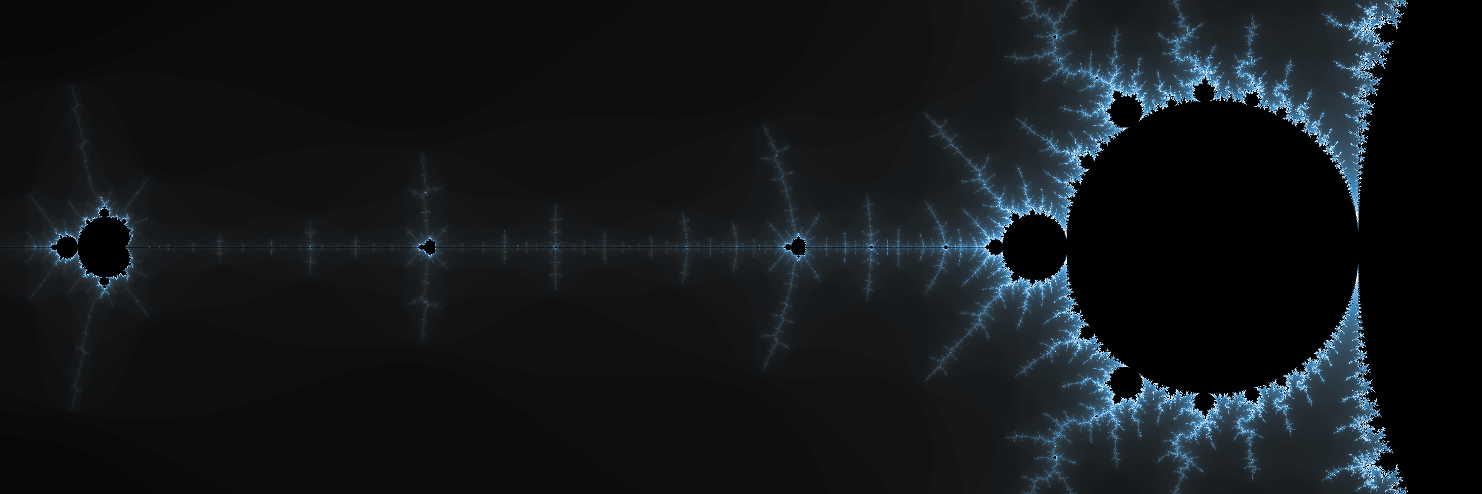
With a suitable rendering mechanism, now we can explore a bit the set, and start looking into interesting portions. We can "zoom in" as much as we want, by defining suitable bounding boxes, and we can increase the detail by increasing the depth. For example, we can take a closer look at the so-called Seahorse valley.

I find this area of the plane truly fascinating, the patterns and depth of it are quite something. To give you an idea, here is a 24 megapixel render, with a depth of 2000 iterations. Go on, click on it, and zoom in to its full size. I'll wait for you here.
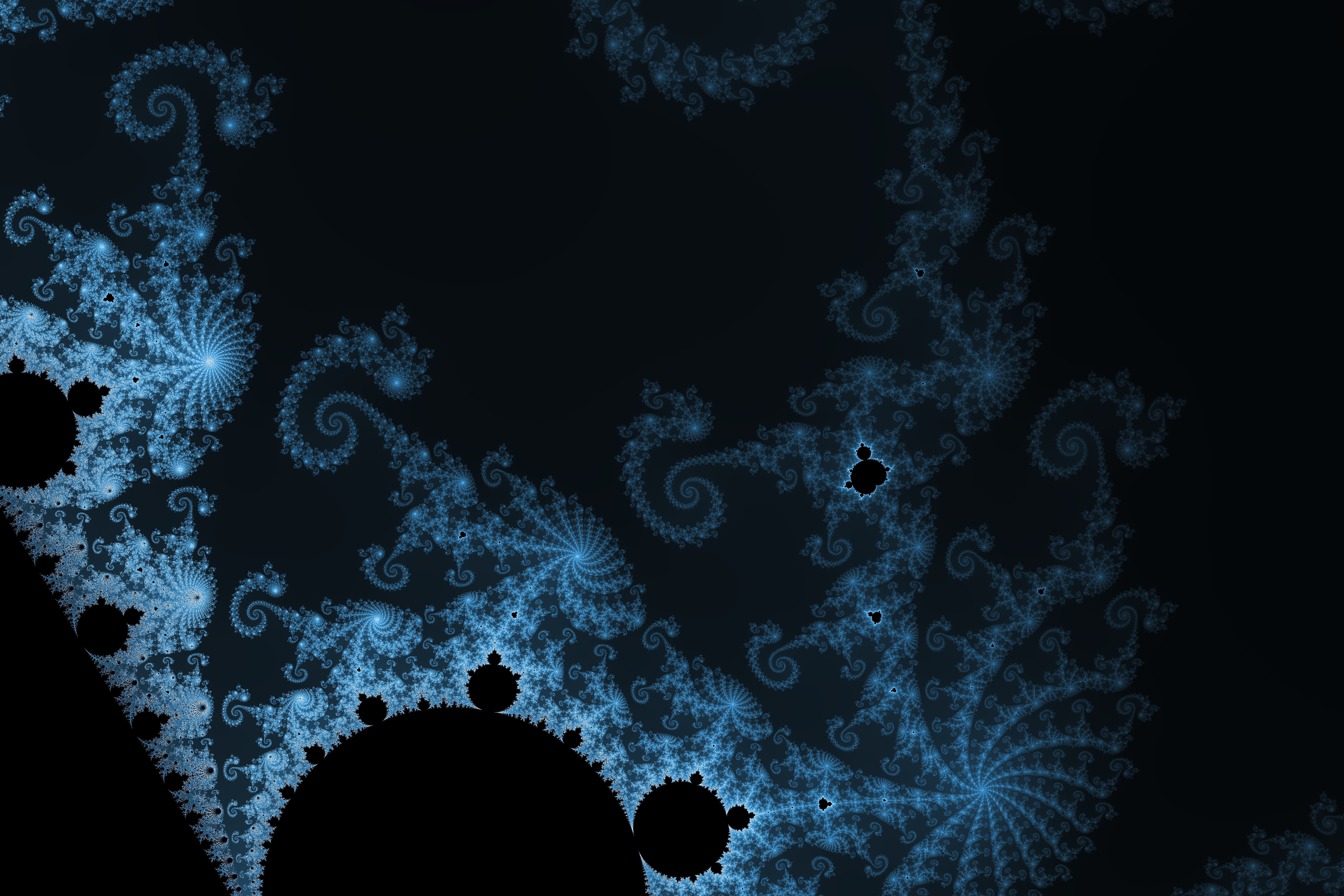
Is that wonderful, or what?
Just One More Thing
In order to appreciate the Mandelbrot set in all its splendor, it would be nice to be able to "fall" into it, with an animation. Given that we have a way to render a view-port onto any area of the plane, it's not much more effort to do it for a set of areas along a path, with different magnification levels.
We will basically start with a target image size (and implied aspect ratio), centered around a point, and with a given surface area on the complex plane. We will then choose another point and another target surface area where the last frame will be centered. All we need to do now is to create the required number of bounding boxes, interpolating position and size over the number of frames to render. Going back to our code:
(ns fractals.animate
  (:require [fractals.mandelbrot :as m]
            [clojure.math.numeric-tower :as nt]))

(defn interpolate-centers [start-point end-point nframes]
  (let [[xs ys] start-point
        [xe ye] end-point
        delta-x (- xe xs)
        delta-y (- ye ys)
        step (/ (Math/sqrt (+ (nt/expt delta-x 2)
                              (nt/expt delta-y 2)))
                nframes)
        theta (Math/atan2  delta-y delta-x)
        next-center (fn [[x y]] [(+ x (* step (Math/cos theta)))
                                 (+ y (* step (Math/sin theta)))])]
    (take (inc nframes) (iterate next-center start-point))))

(defn interpolate-areas [start-area ratio nframes]
  (let [step (nt/expt ratio (/ 1.0 nframes))]
    (take (inc nframes)
          (iterate #(/ % step) start-area))))

(defn bounding-box [aspect-ratio area center]
  (let [[x y] center
        dim-y (nt/sqrt (/ area aspect-ratio))
        dim-x (* dim-y aspect-ratio)
        delta-y (/ dim-y 2)
        delta-x (/ dim-x 2)]
    [[(- x delta-x) (- y delta-y)]
     [(+ x delta-x) (+ y delta-y)]]))

(defn animate-mandelbrot [img-width
                          img-height
                          depth
                          start-point
                          end-point
                          start-area
                          zoom-factor
                          nframes]
  (let [centers (interpolate-centers start-point end-point nframes)
        areas (interpolate-areas start-area zoom-factor nframes)
        aspect-ratio (/ img-width img-height)
        size [img-width img-height]
        b-boxes (map (partial bounding-box aspect-ratio) areas centers)
        names (map (partial format "mb-frame-%04d.png") (range))
        fracs (map #(m/mandelbrot size % depth) b-boxes)]
    (dorun (pmap #(m/do-png %1 size depth %2) fracs names))))
This code technically has a bug, in that when the center position moves across the x axis, the movement mirrors in the rendering (because of how the y axis increases "downwards" on the PNG render), resulting in an angled path, instead of a straight one. Despite this being simple to fix, I'll call this a feature, and leave it in, as it allows for some interesting zooms that would otherwise require a more generic approach to constructing paths .
Here is a full-HD clip of us "falling into the Seahorse Valley". The magnification factor here is 2400x.
That's All, Folks!
I hope you have enjoyed these posts on fractals as much as I enjoyed writing them, they were really a lot of fun to play with! The code can be found on GitHub if you want to play with it.