Enter the Dragon
Fractals have always fascinated me. I remember seeing a render of a Mandelbrot set back in the early 90s (when color screens started being accessible back home), and being completely mesmerized by it. I remember being even more fascinated by seeing a code-golf version of such a renderer, implemented in some 300 bytes of C.
Some days ago I came across the "dragon curve", and decided to give it a go in Clojure, as a way to learn a bit more and have some fun. I implemented it as a Lindenmayer system, which reveals the simplicity behind it.
L-systems are string re-writing systems, and have a set of constants, variables, rules, and a starting axiom. One starts with the axiom, and applies the rules to it. Each rule maps a variable to a new string that substitutes it. Constants are unaffected by the re-write, and remain in place.
In the case of the dragon curve, it can be represented by the following L-system (described nicely in the wiki):
    variables : X Y
    constants : F + −
    start : FX
    rules : X → X+YF+
            Y → −FX−Y
In order to "grow" the dragon, we iterate by applying the rules to the axiom, and then to the result, and so on. For example, after two iterations on the axiom, we have:
| Iteration 1 | ||
| Axiom | FX | |
| Rule for X | FX+YF+ | |
| Iteration 2 | ||
| Rule for X | FX+YF++YF+ | |
| Rule for Y | FX+-FX-YF++-FX-YF+ |
These simple rules, and the simple starting point lead to an increasingly complex string, where structure starts becoming visible. Of course, doing this by hand is extremely tedious, so we can automate it with a bit of Clojure.
We can start by defining the axiom, and the re-writing rules.
  (ns dragon.core
    (:require [hiccup.core :as hiccup]))

  (def start [:F :X])

  (defn rewrite [i]
    (cond
      (= :X i) [:X :+ :Y :F :+]
      (= :Y i) [:- :F :X :- :Y]
      :true [i]))
We can now see what happens when we apply the rules to the axiom:
(map rewrite start)
([:F] [:X :+ :Y :F :+])
This is a bit noisy due to the brackets, but we can see it's the same result we got by iterating by hand. Let's add a bit more functionality:
(defn dragon [segments iter]
  (if (zero? iter)
    segments
    (let [segs (vec (mapcat rewrite segments))]
      (recur segs (- iter 1)))))
Now we can get rid of the extra brackets, and do some more iterations.
(map (partial dragon start) (range 4))
([:F :X]
 [:F :X :+ :Y :F :+]
 [:F :X :+ :Y :F :+ :+ :- :F :X :- :Y :F :+]
 [:F :X :+ :Y :F :+ :+ :- :F :X :- :Y :F :+ :+ :-
  :F :X :+ :Y :F :+ :- :- :F :X :- :Y :F :+])
As we can see in the (slightly reformatted) results, the string's size and complexity keeps increasing.
In order to visualize this fractal, we need some rules on how to interpret it. This is also very simple, and in fact, it is pretty much the same as the turtle graphics that were used in the Logo language.
In this case, we will interpret the F constant as forward (that is, draw a
line in the direction the turtle is facing, and a fixed distance). The + and
- constants will respectively mean right 90 and left 90, that is, to
rotate the turtle by 90 degrees in a given direction. And that's all there is to
it (for now, anyway).
We can again automate this quite easily:
(def pi:2 (/ Math/PI 2))
(def vec:size 3)

(defn points [segments theta acc x y]
  (if (empty? segments)
    acc
    (let [s  (first segments)
          xs (rest segments)]
      (cond
        (or (= s :X) (= s :Y)) (recur xs, theta, acc, x, y)
        (= s :+) (recur xs, (+ theta pi:2), acc, x, y)
        (= s :-) (recur xs, (- theta pi:2), acc, x, y)
        (= s :F) (let [xx (+ x (* vec:size (Math/cos theta)))
                       yy (+ y (* vec:size (Math/sin theta)))
                       new-acc (conj acc (vector xx yy))]
(recur xs, theta, new-acc, xx, yy))))))
We basically go over the generated string, and interpret it according to the
rules described above (ignore constants, draw when we find an F, and turn in
the indicated direction when we find a + or a -. This gives us a list of
points which we can then use to build an SVG polyline.
  (defn render-svg [plot-points]
    (let [width 1000
          height 1000
          xmlns "http://www.w3.org/2000/svg"
          style "stroke:#474674; fill:white;"
          points (apply str (map #(str (first %) "," (second %) " ") plot-points))]
      (hiccup/html [:svg {:width width
                          :height height
                          :xmlns xmlns}
                    [:polyline {:points points
                                :style style}]])))
Here we are using the hiccup library for rendering HTML, and creating a
(potentially very large) polyline element with all the points we defined
above.
Now we can render our dragon and enjoy it in all its glory!
  (let [d    (dragon start 15)
        pts  (points d 0 [] 500 500)
        html (render-svg pts)]
    (spit "dragon15.html" html)

If you are reading this in a modern browser with proper SVG support, you can also open the generated HTML output.
Tidying Up
The code snippets above are fun for playing in the Clojure REPL, but they're don't generalize well, and can be improved upon significantly. In particular, they require some fiddling with the SVG rendering view-port and the starting point of the fractal drawing. I've cleaned up the code a bit, and made it generic so it can support many other L-systems. It now lives on Github, along with some other fractal code that we'll discuss in an upcoming post.
The L-system code itself, if you are interested, lives here.
More Fractal Goodness
Lindenmayer systems can give rise to very many interesting fractals, and many self-similar constructs can also be represented as L-systems. Below you can see some of these.
Box Fractal
axiom : F+F+F+F
rules : F → FF+F+F+F+FF
Five iterations of this system yield this:

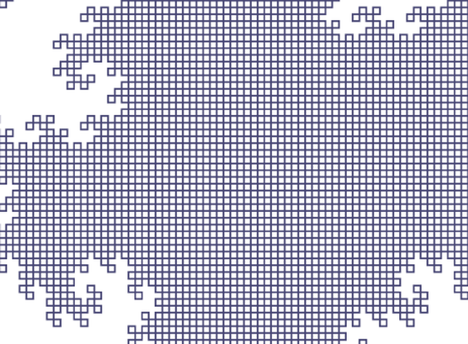
Crystal Fractal
axiom : F+F+F+F
rules : F → FF+F++F+F
Like the Box above, this one also starts with a square (F+F+F+F). Six iterations yield:

Hilbert Curve
axiom : X
rules : X → +YF-XFX-FY+
        Y → -XF+YFY+FX-
The Hilbert curve is a well-known space-filling fractal. It does get quite dense rather quickly. After only 9 iterations, it looks like this.

HTML/SVG version (LARGE FILE!)
Zooming in a bit, we can better discern the structure:

Koch Curve
axiom : F+F+F+F
rules : F → FF+F+F+F+FF
This one also becomes complex very quickly. At four iterations, it looks like this:

Koch Snowflake
axiom : F--F--F
rules : F → F+F--F+F
This is another well-known fractal.

Rings
axiom : F+F+F+F
rules : F → FF+F+F+F+F+F-F
This one is quite eye-catching. After six itertations, we get:

Sierpiński Triangle
axiom : F-G-G
rules : F → F-G+F+G-F
        G → GG
The Sierpiński triangle is another very well known fractal. Unlike the ones seen
above, it has two forward variables, F and G. After 8 iterations, it
results in this:

More to Come!
In this post we have covered the basics of L-system based fractals. There is a
bit more to them, as more "commands" can be embedded in the fractal string, such
as moving the turtle without drawing, and pushing and popping state onto a
stack, to allow for the generation of more complex patterns. The L-system
processing code on Github has some partial support for those, but the renderer
doesn't, so some further work is needed there.
A second part to this incursion into fractals is upcoming. There we'll look into two different types of fractals. The first type is based on affine transformations and stochastic processes, and the second one is the famous Mandelbrot set.